
How to Crosstab Comma Delimited Multi-Select Questions in Excel

When analyzing the results of data you collect through online surveys I always advocate for learning how to analyze your data in Excel/GSheets rather than relying on the data analysis and visualization features in survey tools.
That’s not to say you shouldn’t use the data analysis features in a tool like Survey Monkey or Qualtrics. But if you have a solid understanding of how to work with your data in a raw format, you’ll never be held back by any limitations of the features within the tool itself.
There’s a common data schema for raw quantitative survey data that you’ll see in almost every data export across any survey tool. The format looks something like this.

Example Survey Data Export
In this format every row corresponds to one unique respondent in your survey, and the variables (i.e. questions in the survey) fall across the columns. For the most part this format makes it easy to filter and pivot your dataset, so you can dive deeper into your results and find more meaningful insight.
That said, if you’re new to this format you will find that working with multi-select questions (questions where the respondent can select more than 1 option) can be challenging. The most common way survey tools handle multi-select questions is to spread the response options across multiple columns, where a 1 or 0 (or True/False, Yes/No) indicate whether an option was selected. This is the structure that’s depicted in the image above, see columns F through P, which shows the question response options spread across multiple columns.
This format is common, and necessary because when you have a multi-select question, there’s really no easier way to structure this data for streamlined analysis. That said, this approach presents some challenges. In particular, you can’t easily pivot all the responses across one question in one go, as you have to pivot one option at a time. The good news is that there’s a relatively straightforward solution for this, which is to unpivot your data. This can be done using an Excel add-on called Power Query, or if you’re on a Mac you can use a Google Sheets add-on called Power Tools.
Jon Acampora over at ExcelCampus has a great post/video on how to unpivot multi-select survey data so you can easily analyze it in Excel. So if your survey data is structured in the 1-option-per-column format for your multi-select questions, I highly recommend Jon’s post. I’ve also developed a simple Python script for unpivoting data if you can’t use PowerQuery or Power Tools, which you can access here.
But there’s another format you may encounter that can be even more difficult to work with, where your multi-select question options are all contained within a single cell (i.e. comma delimited). Some survey tools, like Qualtrics, give you the option to export in either the multi or single column format. But other tools don’t always give you the choice. Google Forms is one of them 🙁.
In Google Forms, when you export the raw data any multi-select question will show up in single cell, with all options selected separated by commas. Here’s an example of what raw data from Google Forms looks like (see columns C, D, E and G below).
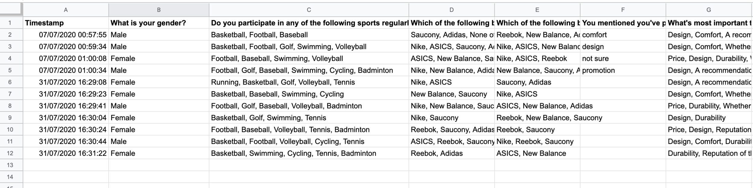
The problem here is that the reporting and visualization features in Google Forms are really limited. There’s no ability to filter or cross-break your data, and the charting / data visualization features are lacking. For the average user who isn’t too savvy in Excel, working with multi-select data in a tool like Google Forms is going to be troublesome.
The good news is that there’s a way to fix this if you want to convert the single column, comma delimited structure to a multi-column structure. Here’s how.
Step 1 - Prepare your data
The first thing you’ll need to do is create new columns in your Excel file, one for each of the options in your multi-select question. So if your multi-select question contains 10 options, you’ll need to create 10 columns.


Step 2 - Add the formula
Now that you’ve created the columns, you’re going to plug in a simple formula that will look for sub-strings (i.e. the individual response options) inside a range, in this case column C in the screen grab above. Here’s the formula (thanks to Dave Bruns over at Exceljet for the helpful post on this formula):
=SUMPRODUCT(COUNTIF(range,"*"substring"*"))>0
The two components you’ll need to set is the range, which is the cell, or cells, that contain the multi-select data (i.e. column C in the above image), as well as the substring, which is the exact text used by the response option.
So, for example, the function for cell D2 will be as follows:
=SUMPRODUCT(COUNTIF($C2,{"*Running*"}))>0
Unfortunately with this function you can’t use a reference cell for the substring, so you will need to manually type in the correct response option for each column (e.g. Running, Basketball, etc). And make sure that the spelling is exactly the same as how it appears in the source column, otherwise the function won’t work properly.
Step 3 - Replicate across all columns
Hopefully the function is working properly for you. If so, you’re ready to copy and paste it across all of the new columns that you’ve created, one for each response option in your multi-select question.
Once this is done the output should look something like this:
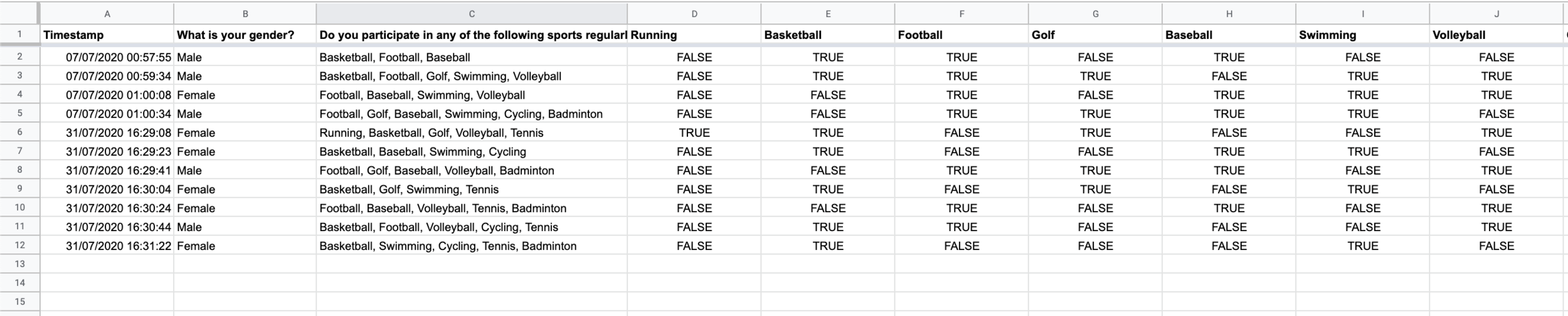
In the new format, you’ll now have 1 column per response option, and the state = “True” indicates that it was selected, while state = “False” indicates that it was not selected.
That’s it!
You can view and download a working version of this dataset with the function here:
In the new, multi-column format there are still some limitations, particularly the fact that you can only pivot one response option at a time. And the solution for that issue is simply to use the unpivot method covered in Jon’s approach that I shared earlier.
I still find it useful to have a version of your dataset in this format, where multi-select questions are structured so response options fall across columns. This format is much more conducive to different forms of custom analysis in Excel, such as cohort or cluster analysis.
That’s all for today. I hope this post was useful, and thanks for reading.
If you enjoyed this article then you’ll love my quantitative market research course. Click the link below for more info.

